Practical: CP2K Parameters
Overview
Teaching: 30 min
Exercises: 45 minQuestions
What QM parameters are there in CP2K and why might we like to change them?
How do we use hybrid functionals such as B3LYP within Gromacs+CP2K?
How can we use a dispersion correction?
How do we ensure the CUTOFF used is fully converged?
How might changes we make affect the performance?
Objectives
Modify the CP2K input to change the basis sets or potentials
Modify the CP2K input to use B3LYP and add dispersion corrections
Do a convergence check for the cutoff energy for the grid
Overview
When using the Gromacs+CP2K interface we have seen that the CP2K input
file containing the CP2K QM parameters is automatically generated and
then passed to CP2K through the interface, which then calculates the
QM/MM energies and forces. The CP2K QM parameters are chosen in order
to usually generate sensible results, for example the BASIS_MOLOPT
basis set as this is commonly used for biological systems, and for the
exchange-correlation (XC) functional PBE is used which is usually a
good compromise between accuracy and computational costs.
However you may want to change some of the input parameters in order to tailor settings to your particular system for greater accuracy, or to use particular functionals, basis sets or potentials. When making these changes it is a good idea to run a standalone CP2K single energy calculation to test the changes and also to monitor how they affect the total energy. Once you are satisfied with the changes the edited CP2K input file can then be used together with the GROMACS+CP2K interface to see the effect on properties of interest.
In this tutorial we will look at making the following changes within the CP2K input settings:
- changing the basis set
- using the B3LYP functional
- adding dispersion correction
- checking the grid convergence
CP2K QM/MM best practice guide
The CP2K best practice guide is a good starting place for changing any QM settings within CP2K. It is available here.
The guide contains information about:
- Understanding the QM input
- Input parameter overview
- The CP2K output
- Basis sets
- Psuedopotentials
- XC functionals
- Dispersion corrections
- Troubleshooting CP2K
Part 1: Changing the basis set
In this exercise we will change the basis set in a CP2K input file. Changing the basis set may be done to improve the accuracy (e.g. using a larger basis set) or reduce the computational costs (smaller basis). Also some basis sets are more suitable in combination with a particular XC functional.
The egfp.inp input file provided uses BASIS_MOLOPT basis
(optimised for molecules). We will change this to the
HFX_BASIS. This will be done because this basis set is suitable
for using with the Hartree-Fock exchange, which is used for B3LYP,
which we will be the focus of the second part of this tutorial.
You can find the input file here:
wget https://github.com/bioexcel/2021-04-22-qmmm-gromacs-cp2k/raw/gh-pages/files/15-cp2k/egfp.inp
And the pdb file is here:
wget https://github.com/bioexcel/2021-04-22-qmmm-gromacs-cp2k/raw/gh-pages/files/15-cp2k/egfp.pdb
In egfp.inp the filename containing the basis set used is defined with the BASIS_SET_FILE_NAME
option, and for each individual element in the &KIND section the BASIS_SET option gives
the basis set for that particular element.
    BASIS_SET_FILE_NAME  BASIS_MOLOPT
    POTENTIAL_FILE_NAME  POTENTIAL
    &KIND H
      ELEMENT H
      BASIS_SET DZVP-MOLOPT-GTH
      POTENTIAL GTH-PBE
    &END KIND
The BASIS_SET option will correspond to one of the basis sets
for the particular element within the basis set file. Note that there is usually no need to
suppy the basis set file directly in your current directory as these are included automatically
from the CP2K data directory path.
On ARCHER2 you can see all the available CP2K basis set files in the following directory:
ls /work/y07/shared/cp2k/cp2k-8.1/data
You can find you basis sets for each element within these files. For example, if you wanted to find all the hydrogen basis sets within BASIS_MOLOPT you could do:
grep ' H ' /work/y07/shared/cp2k/cp2k-8.1/data/BASIS_MOLOPT
TIP:
For more information about basis sets see the QM/MM best practice guide
In the current efgp.inp file the BASIS_MOLOPT basis set filename is used, and the
BASIS_SET for each element is given as DVZP-MOLOPT-GTH. Change these so that
the BASIS_SET_FILE_NAME is set to HFX_BASIS and the BASIS_SET for each element is
TZV2P-GTH. An explaination of how the basis sets are named can be found in the best
practice guide.
You can then run the CP2K job with the following job script.
#!/bin/bash

#SBATCH --job-name=egfp_cp2k
#SBATCH --nodes=1
#SBATCH --tasks-per-node=128
#SBATCH --cpus-per-task=1
#SBATCH --time=00:20:00

#SBATCH --account=ta025
#SBATCH --partition=standard
#SBATCH --qos=standard
#SBATCH --reservation=ta025_167

# Setup the batch environment
module load epcc-job-env

module load cp2k/8.1

export OMP_NUM_THREADS=1

srun --hint=nomultithread cp2k.popt -i egfp.inp > cp2k.out
You will notice that this calculation does a single energy and force calculation for the initial configuration of the system. This is what happens in CP2K during a single MD step when using the GROMACS-CP2K interface.
When the calculation completes a timing report will be printed at the end of cp2k output file.
You should record the total energy and the run time. To extract these from the output you can use:
grep ENERGY cp2k.out
grep 'CP2K   ' cp2k.out
TIP:
The default energy units in CP2K are Hartrees or Atomic Units (au). These can be converted to KJ/mol by multiplying by 2625.5.
This calculation will also generate wave function restart files: GROMACS-RESTART.wfn.
These can be used as an initial guess for the wave function in the self consistent
calculation that CP2K performs, which will help speed up any subsequent
calculations for a similar setup and ensure they reach convergence.
These files will be required for the next exerise.
Rename GROMACS-RESTART.wfn to EGFP-RESTART.wfn to ensure it is not
overwritten.
mv GROMACS-RESTART.wfn EGFP-RESTART.wfn
TIP:
For more information about the CP2K output see the best practice guide
Part 2: Using B3LYP and dispersion corrections
The default exchange-correlation functional used by the interface is PBE, however this can be changed in the CP2K input file. In this example we will change it to use B3LYP. This is a hybrid functional, which means part of it is formed by the exact Hartree Fock exchange, and thus it is more accurate but more computationally expensive than GGA methods such as PBE.
We will also add a dispersion correction to our formulation of the exchange-correlation energy. Here we use the Grimme DFT-D3 method.
To use DFT-D3 the modification will occur within the XC section of the input file. At the moment it looks like this:
    &XC
      DENSITY_CUTOFF     1.0E-12
      GRADIENT_CUTOFF    1.0E-12
      TAU_CUTOFF         1.0E-12
      &XC_FUNCTIONAL PBE
      &END XC_FUNCTIONAL
    &END XC
as we are using PBE as the XC functional. To change to using B3LYP with the DFTD3 dispersion correction you should modify this section as follows:
    &XC
      DENSITY_CUTOFF     1.0E-12
      GRADIENT_CUTOFF    1.0E-12
      TAU_CUTOFF         1.0E-12
         &XC_FUNCTIONAL
      &LYP
         SCALE_C 0.81          ! 81% LYP correlation
      &END
      &BECKE88
         SCALE_X 0.72          ! 72% Becke88 exchange
      &END
      &VWN
         FUNCTIONAL_TYPE VWN3
         SCALE_C 0.19          ! 19% LDA correlation
      &END
      &XALPHA
         SCALE_X 0.08          ! 8%  LDA exchange
      &END
    &END XC_FUNCTIONAL
    &HF
      FRACTION 0.20            ! 20% HF exchange
        &SCREENING
          ! important parameter to get stable HFX calcs
          EPS_SCHWARZ 1.0E-6
          ! needs a good (GGA) initial guess
          SCREEN_ON_INITIAL_P TRUE
        &END
        &INTERACTION_POTENTIAL
          ! for condensed phase systems
          POTENTIAL_TYPE TRUNCATED
          ! should be less than halve the cell
          CUTOFF_RADIUS 4.0
          ! data file needed with the truncated operator
          T_C_G_DATA ./t_c_g.dat
        &END
      &MEMORY
         MAX_MEMORY  1500     ! In MB per MPI rank
      &END
    &END HF

    &VDW_POTENTIAL
         POTENTIAL_TYPE PAIR_POTENTIAL
         &PAIR_POTENTIAL
            PARAMETER_FILE_NAME dftd3.dat
            TYPE DFTD3
            REFERENCE_FUNCTIONAL B3LYP
            R_CUTOFF [angstrom] 16
         &END
      &END VDW_POTENTIAL

    &END XC
These changes incorporate the necessary contributions that make up B3LYP (as mentioned
previously in this course). In addition screening is used to help stabilise the
SCF calculation. EPS_SCHWARZ can be tuned to help with the stabilisation.
You will also need to add the WFN_RESTART_FILE_NAME option in order to read the
correct restart wave function file. This should go in the &DFT section of the
input file, for example after the POTENTIAL_FILE_NAME is specified.
 &DFT
    ...
    POTENTIAL_FILE_NAME  POTENTIAL
    WFN_RESTART_FILE_NAME EGFP-RESTART.wfn
    ...
 &END DFT
You can also change the POTENTIAL used so that the one optimised for BLYP is used rather than the one optimised for PBE since we are no longer using PBE.
    &KIND H
      ELEMENT H
      BASIS_SET TZV2P-GTH
      POTENTIAL GTH-BLYP
    &END KIND
Run the calculation again with the new changes.
Record the total energy and the run time as before, how have these values changed?
Part 3: Cutoff convergence
In this exercise we will look at ensuring that the integration grid
used for mapping the electron density is fine enough. The CUTOFF
keyword in the input file defines the planewave cutoff (default unit
is in Ry) for the finest level of the multi-grid. The higher the
planewave cutoff, the finer the grid. Choosing the value for the
CUTOFF is usually an important step when running a CP2K
calculation and should usually be done whenever changing any of the
main parameters. The CUTOFF should be large enough so that it is
converged with the total energy, however using a too large value will
slow down the calculation without making any improvement in the
accuracy. In the GROMACS-CP2K interface the CUTOFF is set to 450
Ry which should be large enough for most systems, however it is worth
checking this value when making big changes to CP2K parameters.
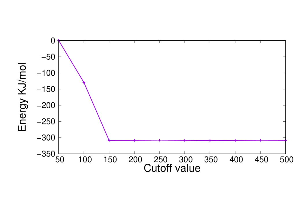
The figure below shows the total energy vs. CUTOFF for our initial input (with PBE).
This demonstrates that the CUTOFF is more than large enough for accurate results.
We are going to repeat this with our modified input file settings in order to check that using a CUTOFF of 450 is still suitable. To do this you will need to edit the CUTOFF value in the input file, run the calculation and then record the total energy, and repeat this process for each value of the cutoff.
You should aim to fill in a table that looks like this:
| CUTOFF | Energy |
|---|---|
| 50 | |
| 100 | |
| 150 | |
| 200 | |
| 250 | |
| 300 | |
| 350 | |
| 400 | |
| 450 | |
| 500 |
How does the CUTOFF vs. total energy compare to the PBE case?
What might be a suitable CUTOFF value to use for our calculation?
Part 4: Looking at performance
We will now look at how changes to the set up may affect the performance of a calculation and how you can optimise the performance when running on multiple nodes.
Functionals
We have seen so far that switching the XC functional from PBE to B3LYP increases the overall run time. B3LYP is more accurate than PBE, but it comes at a cost.
The table below shows the run times found for these methods on a single node of ARCHER2.
| Functional | Run time on 1 node of ARCHER2 (s) |
|---|---|
| PBE | 26.9 |
| B3LYP | 39.9 |
This system has only 19 QM atoms so changing the QM functional may not have a large effect on the run time. For systems with a larger QM region the effect on the run time should be more pronouced.
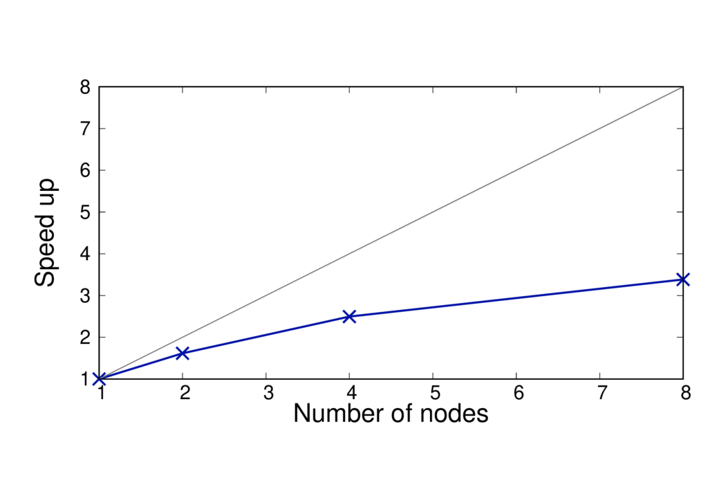
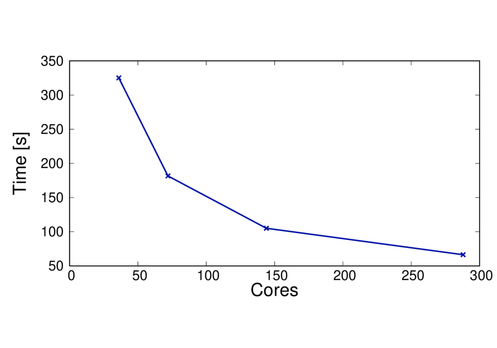
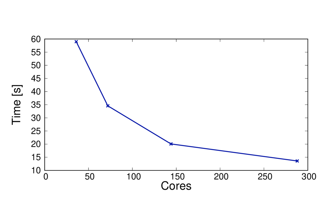
The figures below show the run time and speed up (per MD step) of a different system (CBD_PHY) with 68 QM atoms. The PBE (GGA) and PBE0 (hybrid) functionals are shown.
The results are reported for Cirrus which has 36 cores per node. No multi-threading is used.
CBD_PHY - PBE
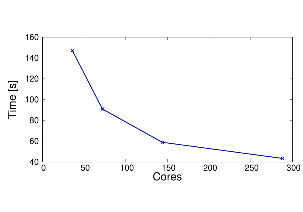
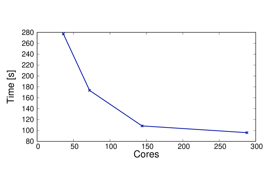
CBD_PHY - PBE0
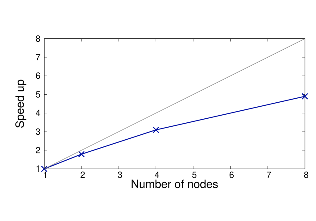
Key observations
- The run time per MD step is almost doubled when using PBE0.
- The speed up is greater as the method is more complex and can benefit from using more cores.
- When switching to a hybrid functional it makes sense to run on more nodes.
QM region size
The QM region size will affect the performance. More QM atoms will make the calculation more computationally expensive. The figures below show the run time and speed up per MD step for the same system but with 19 and 253 QM atoms.
The results are shown for Cirrus and each run uses 6 threads per MPI process.
ClC 19 QM atoms - BLYP
ClC 253 QM atoms - BLYP
Key observations
- The run time per MD step is much larger for the larger QM system
Using multiple threads
Using threading in a calculation (i.e MPI+OpenMP) may improve the performance. However the optimum number of threads will depend on many things such as the machine architecture, the type of calculation and your system size. As a general rule the number of threads per MPI process has to be chosen so that it evenly divides the number of MPI processes on a node, whilst ensuring that threads sharing memory are in the same NUMA region. The total number of MPI processes will need to be set so that the number of threads per process multiplied by the number of MPI processes gives the total number of cores requested.
The run times per MD step for different systems with different threading configurations are shown in the figures below.
CBD_PHY - PBE
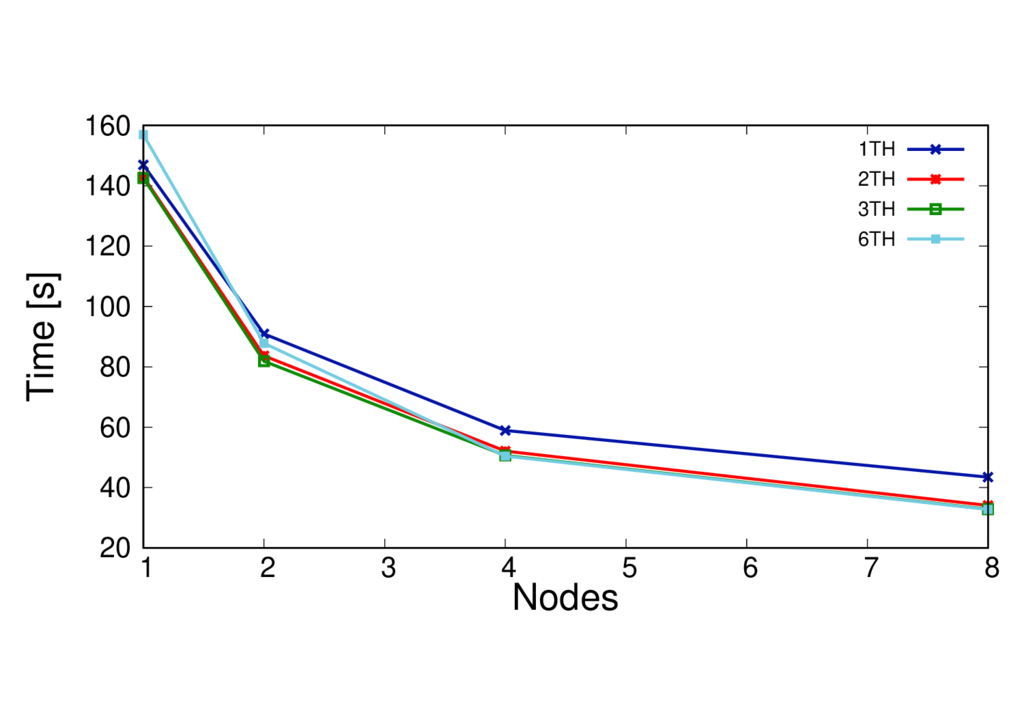
ClC 253 QM atoms - BLYP
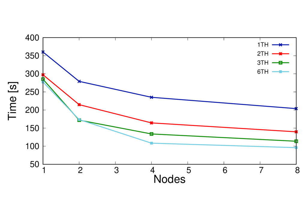
Key observations
- In this case using more threads per process is beneficial
- This is particularly the case on more nodes - threading helps extend the scaling
- The best number of threads to use for performace will depend on many things - it is best to test this.
Key Points
How to change CP2K parameters and make sensible choices
Using hybrid functionals and dispersion corrections
How to check the cutoff convergence
Available basis sets and potentials
QM/MM performance considerations