Practical: GROMACS + CP2K Part I
Overview
Teaching: 25 min
Exercises: 50 minQuestions
What is GROMACS-CP2K QMMM Interface?
How it could be used?
Objectives
Getting started with GROMACS-CP2K Interface
Learning how to prepare your system for a simple QM calculation
Umbrella sampling using GROMACS-CP2K Interface
Preparing for the tutorial
Everything, which is written inside the gray box are a commands, that should be executed in the terminal window, string-by-string, each following with the ENTER button.
Please note that <...> in the commands means, that everything, including <> symbols, must be replaced with your own specific information. Be careful!
Helpful utilities and commands
Some exercises will require usage of
lessLinux tool for looking up into the content of files. In case you are not familiar with it, here is a short list of hotkeys, which could be used inside LESS editor:
- q – exit
- / – search for a pattern which will take you to the next occurrence
- n – for next match in forward
- N (SHIFT+n) – for previous match in backward
- g – go to the start of file
- G (SHIFT+g) – go to the end of file
All exercises will require you to submit job for computing using
sbatch run.shcommand. To check status of your job following commands would be useful.
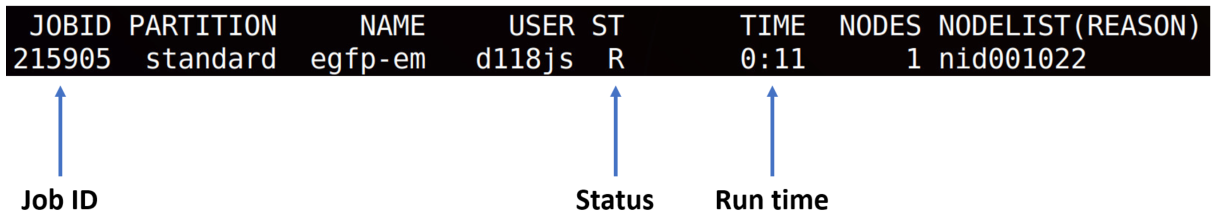
squeue -u <your login name>- checks status of all your jobs. Output will look like that:scancel <JOBID>will remove the job, if you occasionally submitted it.
Setting up tutorial environment
Let’s start the tutorial with the following steps
- Execute commands in the terminal:
module load gromacs-cp2k
cd /work/ta025/ta025/<your login name>
git clone https://github.com/bioexcel/2021-04-22-gromacs-cp2k-tutorial.git tutorial - And go to the tutorial directory
cd tutorial
Exercise 1: Setting up simple QM system
1) Go to nma directory:
cd nma
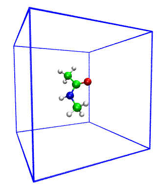
In the directory located forcefield and nma.pdb file with a geometry of simple compuond N-Methylacetamide (NMA)
You can download it and inspect structure with VMD or PyMOL.
2) Make topology for the system using the following command:
gmx_cp2k pdb2gmx -f nma.pdb
choose the following forcefield and water model:
Select the Force Field:
From current directory:
1: CHARMM36 all-atom force field (March 2019)
....
....
Select the Water Model:
1: TIP3P       TIP 3-point, recommended, by default uses CHARMM TIP3 with LJ on H
Files topol.top, conf.gro and posre.itp should appear in the directory
3) Look into Gromacs input file em.mdp:
less em.mdp
The following lines contain QMMM MdModule options:
; CP2K QMMM parameters
qmmm-active              = true   ; Activate QMMM MdModule
qmmm-qmgroup             = System ; Index group of QM atoms
qmmm-qmmethod            = PBE    ; Method to use
qmmm-qmcharge            = 0      ; Charge of QM system
qmmm-qmmultiplicity      = 1      ; Multiplicity of QM system
4) Lets perform energy minimization first for that molecule using QMMM interface
Generate Gromacs-CP2K simulation file:
gmx_cp2k grompp -f em.mdp -p topol.top -c conf.gro -o nma-em.tpr
files nma-em.tpr, nma-em.inp and nma-em.pdb should appear in the directory
5) Run QMMM simulation:
sbatch run-em.sh
6) While job is running you can check the content of nma-em.inp
less nma-em.inp
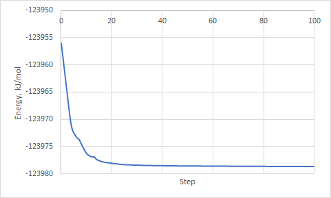
7) At the end of the job use the following command to extract potential energy:
gmx_cp2k energy
and choose 5 Potential
File energy.xvg should appear in the directory. It contains data with Potential energy (kJ/mol) against optimization step. You can open it in Grace or copy data into any other software (i.e. Excel).
8) Next we will perform short (100 fs) MD simulation with QM. At first look into the md-nvt.mdp file:
less md-nvt.mdp
It contains parameters for performing dynamics with QM forces in the NVT ensemble at 300K
9) Generate Gromacs-CP2K simulation file:
gmx_cp2k grompp -f md-nvt.mdp -p topol.top -c conf.gro -o nma-nvt.tpr
files nma-nvt.tpr, nma-nvt.inp and nma-nvt.pdb should appear in the directory
10) Run QMMM simulation:
sbatch run-nvt.sh
11) At the end of the simulation you can download trajectory file traj.trr and render it using your favorite software (e.g. VMD, PyMOL).
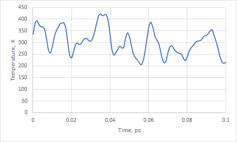
Also you could check temperature as a function of time with the following command:
gmx_cp2k energy
and choose 9 Temperature
File energy.xvg will contain data about Temperature (K) against simulation time (ps).
Notice, how temperature fluctuates around 300K.
Exercise 2: Umbrella sampling simulation with QMMM MdModule
1) Go to stilbene_vacuum directory:
cd ../stilbene_vacuum
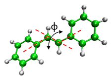
2) Look up in the table and pick-up starting structure and dihedral angle value:
| Structure | Dihedral angle, φ |
|---|---|
| md-equilb1.gro | -180 |
| md-equilb2.gro | -173 |
| md-equilb3.gro | -166 |
| md-equilb4.gro | -159 |
| md-equilb5.gro | -152 |
| md-equilb6.gro | -145 |
| md-equilb7.gro | -138 |
| md-equilb8.gro | -131 |
| md-equilb9.gro | -124 |
| md-equilb10.gro | -117 |
| md-equilb11.gro | -110 |
| md-equilb12.gro | -103 |
| md-equilb13.gro | -96 |
| md-equilb14.gro | -89 |
| md-equilb15.gro | -82 |
| md-equilb16.gro | -75 |
| md-equilb17.gro | -68 |
| md-equilb18.gro | -61 |
| md-equilb19.gro | -54 |
| md-equilb20.gro | -47 |
| md-equilb21.gro | -40 |
| md-equilb22.gro | -33 |
| md-equilb23.gro | -26 |
| md-equilb24.gro | -19 |
| md-equilb25.gro | -12 |
| md-equilb26.gro | -5 |
| md-equilb27.gro | 2 |
| md-equilb28.gro | 9 |
| md-equilb29.gro | 16 |
| md-equilb30.gro | 23 |
3) Copy chosen starting structure:
cp eq_gro/<your starting gro> ./conf.gro
4) Modify Gromacs input file qmmm_md_umbrella.mdp with value of your chosen Dihedral angle:
sed -i "s/@umbr@/<your dihedral angle>/" qmmm_md_umbrella.mdp
You can also modify pull-coord1-init option in the qmmm_md_umbrella.mdp file with vim or any other editor.
5) Add group of atoms which will be treated with QM to the index file (in that case all atoms are QM):
gmx_cp2k make_ndx -f conf.gro -n index.ndx
> 0
> name 7 QMatoms
> q
6) Generate Gromacs-CP2K simulation file:
gmx_cp2k grompp -f qmmm_md_umbrella.mdp -p topol.top -c conf.gro -n index.ndx -o stilbene.tpr
files stilbene.tpr, stilbene.inp and stilbene.pdb should appear in the directory
7) Run QMMM simulation:
sbatch run.sh
8) While job is running you can check the content of stilbene.inp
less stilbene.inp
and of qmmm_md_umbrella.mdp
less qmmm_md_umbrella.mdp
9) At the end of the job copy files stilbene.tpr and pullx.tpr into the shared directory. Beware as you need to append filenames with <your number> when copying:
cp stilbene.tpr /work/ta025/ta025/shared/tutorial/umbrella/stilbene<your number>.tpr
cp pullx.xvg /work/ta025/ta025/shared/tutorial/umbrella/pullx<your number>.xvg
Check also pull.xvg file:
less pullx.xvg
It contains information about chosen coordinate dynamics over the simulation trajectory. By performing that sampling over the many points along reaction coordinate and gathering all *.tpr and pullx.xvg files you could produce free-energy profile of the reaction with gmx_cp2k wham tool.
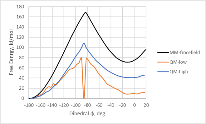
10) After gathering files from all participants, trainer will generate free energy profile /work/ta011/ta011/shared/tutorial/umbrella/profile.xvg
It contains data about Free energy (kJ/mol) against Dihedral angle (deg). You can download and open it in Grace or copy data into any other software (i.e. Excel).
11) Check the free energy profiles generated from 100 steps (100 fs) and 10000 steps (10 ps) of QMMM MD simulation for each frame from the eq_gro directory: profile-100fs.xvg and profile-10ps.xvg. You can open them with Grace or copy data into any other software (i.e. Excel).
Key Points
QM simulation could be activated by adding several parameters into the mdp file
Most of the simulation techniques from GROMACS are available also within QMMM
When doing advanced sampling with QMMM one should be aware of the distribution and final profile quality